R Cheatsheet (tidy version)
- Week 0
- Vectors
- Create a vector
- Creating a vector from a sequence
- Length of a vector
- Summarizing a numeric vector
- Means, median, sums, min, max
- Ranges of a vector
- Subsetting a vector
- Subsetting by a logical vector
- Subsetting accidents
- Subsetting to the first 5 values
- Subsetting to the last value in a vector
- Modifying values in a vector
- Arithmetic on vectors
- Character vectors
- Data frames
- Vectors
- Week 1
- Week 2
- Week 3
- Week 4
- Week 5
- Week 6
- Week 7
- Week 8
- Week 9
- Week 11
Week 0
Vectors
Create a vector
Use the c() function for concatenate.
x <- c(2.2, 6.2, 1.2, 5.5, 20.1)Creating a vector from a sequence
The seq() function will create a sequence from a starting point to an ending point. If you specify the by argument, you can skip values. For instance, if we wanted a vector of all presidential election years from 1788 until 2020, we would use:
pres_elections <- seq(from = 1788, to = 2020, by = 4)
pres_elections
## [1] 1788 1792 1796 1800 1804 1808 1812 1816 1820 1824 1828 1832 1836 1840 1844 1848 1852
## [18] 1856 1860 1864 1868 1872 1876 1880 1884 1888 1892 1896 1900 1904 1908 1912 1916 1920
## [35] 1924 1928 1932 1936 1940 1944 1948 1952 1956 1960 1964 1968 1972 1976 1980 1984 1988
## [52] 1992 1996 2000 2004 2008 2012 2016 2020If we want to a sequence from a to b counting by 1s, we can use the a:b shorthand:
2014:2020## [1] 2014 2015 2016 2017 2018 2019 2020Length of a vector
length(x)## [1] 5Summarizing a numeric vector
The summary function will give you some summary statistics about a vector:
summary(pres_elections)## Min. 1st Qu. Median Mean 3rd Qu. Max.
## 1788 1846 1904 1904 1962 2020Means, median, sums, min, max
There are various simple summary functions for specific summaries.
mean(x)## [1] 7.04median(x)## [1] 5.5sum(x)## [1] 35.2Ranges of a vector
You can easily get the smallest and largest values of a vector with min, max, and range.
min(x)## [1] 1.2max(x)## [1] 20.1## get both in one vector
range(x)## [1] 1.2 20.1Subsetting a vector
To access a single element of a vector by position in the vector, use the square brackets []:
x[2]## [1] 6.2If you want to access more than one element of a vector, put a vector of the positions you want to access in the brackets:
x[c(2, 5)]## [1] 6.2 20.1Subsetting by a logical vector
The last two approaches selected subsets by position (“give me the 2nd and 5th element of this vector”). Many times, we will want to select the values of a vector that meet some logical condition. To achieve this, we can put a logical vector the same length as the vector being subsetted in the square [] brackets with TRUE or FALSE indicating if each entry should or should not be included in the subset. For instance, we can recreate the x[c(2, 5)] subset with the following:
x[c(FALSE, TRUE, FALSE, FALSE, TRUE)]## [1] 6.2 20.1More usefully, we can create logical vectors from expressions to get all values from the vector that meet some condition:
x[x > 5]## [1] 6.2 5.5 20.1Gotcha: if your logical subsetting vector that is shorter than the length of the vector being subsetted, R will implicitly repeat the logical vector to the right length. So these two commands give the same output:
x[c(TRUE, FALSE)]## [1] 2.2 1.2 20.1x[c(TRUE, FALSE, TRUE, FALSE, TRUE)]## [1] 2.2 1.2 20.1If your logical subsetting vector is longer than the vector being subsetted, you will get NA values for the values beyond the correct length:
x[c(TRUE, TRUE, TRUE, FALSE, TRUE, TRUE, TRUE)]## [1] 2.2 6.2 1.2 20.1 NA NASubsetting accidents
If you try to access an element past the length of the vector, it will return a missing value NA:
x[10]## [1] NAIf you accidentally subset a vector by NA (the missing value), you get the vector back with all its entries replaced by NA:
x[NA]## [1] NA NA NA NA NASometimes you’ll notice that a vector or data frame you’ve been messing with all of a sudden has lots of missing values (maybe whole rows of them). Usually the culprit in that case is some errant missing value in a subset.
Subsetting to the first 5 values
pres_elections[1:5]## [1] 1788 1792 1796 1800 1804head(pres_elections, n = 5)## [1] 1788 1792 1796 1800 1804Subsetting to the last value in a vector
The length function gives us the number of positions in the vector and so it is also the last position. You can also use the tail function.
pres_elections[length(pres_elections)]## [1] 2020tail(pres_elections, n = 1)## [1] 2020Modifying values in a vector
Let’s say you want to modify one value in your vector. You can combine the square bracket subset [] with the assignment operator <- to replace a particular value:
x## [1] 2.2 6.2 1.2 5.5 20.1x[3] <- 50.3
x## [1] 2.2 6.2 50.3 5.5 20.1You can replace multiple values at the same time by using a vector for subsetting:
x## [1] 2.2 6.2 50.3 5.5 20.1x[1:2] <- c(-1.3, 42)
x## [1] -1.3 42.0 50.3 5.5 20.1If the replacement vector (the right-hand side) is shorter than what you are assigning to (the left-hand side), the values will “recycle” or repeat as necessary:
x[1:2] <- 3.2
x
## [1] 3.2 3.2 50.3 5.5 20.1x[1:4] <- c(1.2, 2.4)
x## [1] 1.2 2.4 1.2 2.4 20.1Gotcha: if the right-hand side length is not a multiple of the left-hand side length, R will do the replacement and truncate things correctly, but will complain and give a warning:
x[1:3] <- c(0.5, 1.5)## Warning in x[1:3] <- c(0.5, 1.5): number of items to replace is not a multiple of
## replacement lengthx## [1] 0.5 1.5 0.5 2.4 20.1Usually if you get this warning in Gov 51, something has gone wrong and you should check your code. (That’s a more general rule about warnings in Gov 51.)
Arithmetic on vectors
You can perform simple arithmetic on vectors and it will apply to each element:
x## [1] 0.5 1.5 0.5 2.4 20.1x * 10## [1] 5 15 5 24 201You can also take apply arithmetic on multiple vectors that are the same lengths. Suppose we have two vectors of test scores for 5 students. We can calculate the change in their scores with:
score_1 <- c(88, 95, 92, 75, 82)
score_2 <- c(90, 92, 97, 81, 85)
score_2 - score_1
## [1] 2 -3 5 6 3Of course, we could also save that vector for future use:
score_change <- score_2 - score_1
mean(score_change)
## [1] 2.6Character vectors
You can also create a vector of characters (words, letters, punctuation, etc):
jedi <- c("Yoda", "Obi-Wan", "Luke", "Leia", "Rey")Note for vectors, you cannot mix characters and numbers in the same vector. If you add a single character element, the whole vector gets converted.
## output is numeric
x
## [1] 0.5 1.5 0.5 2.4 20.1## output is now character
c(x, "hey")## [1] "0.5" "1.5" "0.5" "2.4" "20.1" "hey"Data frames
Reading in CSV files
You can import data into R using the read.csv() function.
my_data <- read.csv("data/mydata.csv")Troubleshooting: if you get an error trying to load data, double check the name of the file you are trying to load and make sure that the csv file exists where you think it does. You can always look at the Files pane of RStudio to look in a data folder to see what the contents are and what the names of the files are you are trying to import.
Reading in RData files
You can read files with an .RData extension with the load() function:
load("data/mydata.RData")With the load() function, you don’t actually assign its output to anything. An .RData file contains R objects (vectors, data frame, etc) and when you load it, those objects are dumped into your R environment.
Dimensions of a data frame
The cars data frame is built into R and so you can access it without loading any files. To get the dimensions, you can use dim(), nrow(), and ncol().
dim(mtcars)## [1] 32 11nrow(mtcars)## [1] 32ncol(mtcars)## [1] 11Accessing variables/columns
You can grab each column/variable from the data frame use the $, turning it into a vector:
mtcars$wt## [1] 2.620 2.875 2.320 3.215 3.440 3.460 3.570 3.190 3.150 3.440 3.440 4.070 3.730 3.780
## [15] 5.250 5.424 5.345 2.200 1.615 1.835 2.465 3.520 3.435 3.840 3.845 1.935 2.140 1.513
## [29] 3.170 2.770 3.570 2.780You can now treat this just like a vector, with the subsets and all.
mtcars$wt[1]## [1] 2.62Subset to the first/last k rows of a data frame
head(mtcars)## mpg cyl disp hp drat wt qsec vs am gear carb
## Mazda RX4 21.0 6 160 110 3.90 2.620 16.46 0 1 4 4
## Mazda RX4 Wag 21.0 6 160 110 3.90 2.875 17.02 0 1 4 4
## Datsun 710 22.8 4 108 93 3.85 2.320 18.61 1 1 4 1
## Hornet 4 Drive 21.4 6 258 110 3.08 3.215 19.44 1 0 3 1
## Hornet Sportabout 18.7 8 360 175 3.15 3.440 17.02 0 0 3 2
## Valiant 18.1 6 225 105 2.76 3.460 20.22 1 0 3 1tail(mtcars)## mpg cyl disp hp drat wt qsec vs am gear carb
## Porsche 914-2 26.0 4 120.3 91 4.43 2.140 16.7 0 1 5 2
## Lotus Europa 30.4 4 95.1 113 3.77 1.513 16.9 1 1 5 2
## Ford Pantera L 15.8 8 351.0 264 4.22 3.170 14.5 0 1 5 4
## Ferrari Dino 19.7 6 145.0 175 3.62 2.770 15.5 0 1 5 6
## Maserati Bora 15.0 8 301.0 335 3.54 3.570 14.6 0 1 5 8
## Volvo 142E 21.4 4 121.0 109 4.11 2.780 18.6 1 1 4 2Subsetting a data frame by rows/columns
Subsetting a data frame means selecting certain rows or columns. In tidyverse, you can do this with the filter() function for selecting rows and the select() function for selecting columns. Here we pipe the selections into head() to show the first few rows. You could also use the dplyr::slice_head function
mtcars %>%
  select(mpg, wt) %>%
  head()
## mpg wt
## Mazda RX4 21.0 2.620
## Mazda RX4 Wag 21.0 2.875
## Datsun 710 22.8 2.320
## Hornet 4 Drive 21.4 3.215
## Hornet Sportabout 18.7 3.440
## Valiant 18.1 3.460To select the cars with eight cylinders:
mtcars %>%
  filter(cyl == 8)
## mpg cyl disp hp drat wt qsec vs am gear carb
## Hornet Sportabout 18.7 8 360.0 175 3.15 3.440 17.02 0 0 3 2
## Duster 360 14.3 8 360.0 245 3.21 3.570 15.84 0 0 3 4
## Merc 450SE 16.4 8 275.8 180 3.07 4.070 17.40 0 0 3 3
## Merc 450SL 17.3 8 275.8 180 3.07 3.730 17.60 0 0 3 3
## Merc 450SLC 15.2 8 275.8 180 3.07 3.780 18.00 0 0 3 3
## Cadillac Fleetwood 10.4 8 472.0 205 2.93 5.250 17.98 0 0 3 4
## Lincoln Continental 10.4 8 460.0 215 3.00 5.424 17.82 0 0 3 4
## Chrysler Imperial 14.7 8 440.0 230 3.23 5.345 17.42 0 0 3 4
## Dodge Challenger 15.5 8 318.0 150 2.76 3.520 16.87 0 0 3 2
## AMC Javelin 15.2 8 304.0 150 3.15 3.435 17.30 0 0 3 2
## Camaro Z28 13.3 8 350.0 245 3.73 3.840 15.41 0 0 3 4
## Pontiac Firebird 19.2 8 400.0 175 3.08 3.845 17.05 0 0 3 2
## Ford Pantera L 15.8 8 351.0 264 4.22 3.170 14.50 0 1 5 4
## Maserati Bora 15.0 8 301.0 335 3.54 3.570 14.60 0 1 5 8We can use the slice() function. For example, to get the 5th through 10th rows:
mtcars %>%
  slice(5:10)
## mpg cyl disp hp drat wt qsec vs am gear carb
## Hornet Sportabout 18.7 8 360.0 175 3.15 3.44 17.02 0 0 3 2
## Valiant 18.1 6 225.0 105 2.76 3.46 20.22 1 0 3 1
## Duster 360 14.3 8 360.0 245 3.21 3.57 15.84 0 0 3 4
## Merc 240D 24.4 4 146.7 62 3.69 3.19 20.00 1 0 4 2
## Merc 230 22.8 4 140.8 95 3.92 3.15 22.90 1 0 4 2
## Merc 280 19.2 6 167.6 123 3.92 3.44 18.30 1 0 4 4If we pass a vector of integers to the select function, we will get the variables corresponding to those column positions. So to get the first through third columns:
mtcars %>%
  select(1:3) %>%
  head()
## mpg cyl disp
## Mazda RX4 21.0 6 160
## Mazda RX4 Wag 21.0 6 160
## Datsun 710 22.8 4 108
## Hornet 4 Drive 21.4 6 258
## Hornet Sportabout 18.7 8 360
## Valiant 18.1 6 225Summarizing a data frame
If you call summary() a data frame, it produces applies the vector version of the summary command to each column:
summary(mtcars)## mpg cyl disp hp drat
## Min. :10.40 Min. :4.000 Min. : 71.1 Min. : 52.0 Min. :2.760
## 1st Qu.:15.43 1st Qu.:4.000 1st Qu.:120.8 1st Qu.: 96.5 1st Qu.:3.080
## Median :19.20 Median :6.000 Median :196.3 Median :123.0 Median :3.695
## Mean :20.09 Mean :6.188 Mean :230.7 Mean :146.7 Mean :3.597
## 3rd Qu.:22.80 3rd Qu.:8.000 3rd Qu.:326.0 3rd Qu.:180.0 3rd Qu.:3.920
## Max. :33.90 Max. :8.000 Max. :472.0 Max. :335.0 Max. :4.930
## wt qsec vs am gear
## Min. :1.513 Min. :14.50 Min. :0.0000 Min. :0.0000 Min. :3.000
## 1st Qu.:2.581 1st Qu.:16.89 1st Qu.:0.0000 1st Qu.:0.0000 1st Qu.:3.000
## Median :3.325 Median :17.71 Median :0.0000 Median :0.0000 Median :4.000
## Mean :3.217 Mean :17.85 Mean :0.4375 Mean :0.4062 Mean :3.688
## 3rd Qu.:3.610 3rd Qu.:18.90 3rd Qu.:1.0000 3rd Qu.:1.0000 3rd Qu.:4.000
## Max. :5.424 Max. :22.90 Max. :1.0000 Max. :1.0000 Max. :5.000
## carb
## Min. :1.000
## 1st Qu.:2.000
## Median :2.000
## Mean :2.812
## 3rd Qu.:4.000
## Max. :8.000Week 1
For this section, we’ll use the social data from QSS, which is the social pressure mailer for voter turnout experiment.
data("social", package = "qss")Getting counts and cross-tabs
Get counts of each value in a variable
You can use the group_by and summarize functions to get counts within levels of a single variable:
social %>%
  group_by(primary2004) %>%
  summarize(n = n())
## `summarise()` ungrouping output (override with `.groups` argument)## # A tibble: 2 x 2
## primary2004 n
## <int> <int>
## 1 0 183098
## 2 1 122768A simpler way to perform the same action is to use the count() function:
social %>% count(primary2004)## primary2004 n
## 1 0 183098
## 2 1 122768Cross-tabulation
When grouping by two variables, this same approach will return counts for each combination of the two vectors:
social %>%
  group_by(primary2004, primary2006) %>%
  summarize(n = n())
## `summarise()` regrouping output by 'primary2004' (override with `.groups` argument)## # A tibble: 4 x 3
## # Groups: primary2004 [2]
## primary2004 primary2006 n
## <int> <int> <int>
## 1 0 0 137162
## 2 0 1 45936
## 3 1 0 73199
## 4 1 1 49569And with count:
social %>% count(primary2004, primary2006)## primary2004 primary2006 n
## 1 0 0 137162
## 2 0 1 45936
## 3 1 0 73199
## 4 1 1 49569To put these into a cross-tab format, you need to put one of variables into the columns using pivot_wider:
social %>%
  group_by(primary2004, primary2006) %>%
  summarize(n = n()) %>%
  pivot_wider(names_from = primary2006, values_from = n)
## `summarise()` regrouping output by 'primary2004' (override with `.groups` argument)## # A tibble: 2 x 3
## # Groups: primary2004 [2]
## primary2004 `0` `1`
## <int> <int> <int>
## 1 0 137162 45936
## 2 1 73199 49569To get slightly nicer column names in this crosstab, we can use names_prefix:
social %>%
  group_by(primary2004, primary2006) %>%
  summarize(n = n()) %>%
  pivot_wider(
    names_from = primary2006,
    values_from = n,
    names_prefix = "primary2006_"
  )
## `summarise()` regrouping output by 'primary2004' (override with `.groups` argument)## # A tibble: 2 x 3
## # Groups: primary2004 [2]
## primary2004 primary2006_0 primary2006_1
## <int> <int> <int>
## 1 0 137162 45936
## 2 1 73199 49569Converting counts to proportions
You can convert any count to a proportion fairly easily using the nrow() command:
social %>%
  group_by(primary2004) %>%
  summarize(prop = n() / nrow(social))
## `summarise()` ungrouping output (override with `.groups` argument)## # A tibble: 2 x 2
## primary2004 prop
## <int> <dbl>
## 1 0 0.599
## 2 1 0.401Controlling output
Rounding numbers
R often gives you way more significant digits than you need to display. You can always pass a vector or number to round() to display/print only a certain number of digits:
p_counts <- social %>%
  group_by(primary2006) %>%
  summarize(prop = n() / nrow(social)) %>%
  pull(prop, name = primary2006)
## `summarise()` ungrouping output (override with `.groups` argument)p_counts## 0 1
## 0.6877554 0.3122446round(p_counts, digits = 2)## 0 1
## 0.69 0.31This is useful in R Markdown files when you want to access a particular value in text as `r mean(social$primary2006)` which would be 0.3122446. You can instead use `r round(mean(social$primary2006), 2)` to get 0.31.
Logicals
Logical vectors
Logical vectors are just vectors that only contain the special R values TRUE or FALSE.
c(TRUE, FALSE, TRUE, TRUE, FALSE)## [1] TRUE FALSE TRUE TRUE FALSETRUE/FALSE are case sensitive
You could but never should shorten TRUE to T and FALSE to F. It’s easy for this shortening to go wrong so better just to spell out the full word. Also not that this is case-sensitive, and this will produce an error:
true## Error in eval(expr, envir, enclos): object 'true' not foundTrue## Error in eval(expr, envir, enclos): object 'True' not foundfalse## Error in eval(expr, envir, enclos): object 'false' not foundConverting logicals to numerics
Like numeric and character vectors, you cannot mix these types with other values. But if you treat a logical vector like a numeric and apply a function to it, R will usually silent convert the logical to a numeric with TRUE being assigned to 1 and FALSE being assigned to 0. You can see this explicitly by passing a logical vector to the as.numeric function:
as.numeric(c(TRUE, FALSE, TRUE, TRUE, FALSE))## [1] 1 0 1 1 0The number and proportion of TRUE values
Because of the conversion mentioned above, passing a logical vector to the sum() function (which adds all of the entries together) will return the number of true values in the vector:
sum(c(TRUE, FALSE, TRUE, TRUE, FALSE))## [1] 3The mean() function will give the proportion of TRUE values in the vector:
mean(c(TRUE, FALSE, TRUE, TRUE, FALSE))## [1] 0.6and/or statements with logicals
We often combine logical statements using AND (&) and OR (|) in R. For AND statements, both expressions have to be true for the whole expression to be true:
TRUE & FALSE,FALSE & TRUE, andFALSE & FALSEareFALSETRUE & TRUEisTRUE
For OR statements, either statement being true makes the whole expression true:
TRUE | FALSE,FALSE | TRUE, andTRUE | TRUEareTRUEFALSE | FALSEisFALSE
You can also use these to compare two logical vectors:
## Apply "or" statement to each pair of elements
c(TRUE, FALSE, TRUE, TRUE, FALSE) | c(TRUE, TRUE, FALSE, FALSE, FALSE)
## [1] TRUE TRUE TRUE TRUE FALSE# Apply "and" statement to each pair of elements
c(TRUE, FALSE, TRUE, TRUE, FALSE) & c(TRUE, TRUE, FALSE, FALSE, FALSE)## [1] TRUE FALSE FALSE FALSE FALSEComparing objects
There are several relational operators that allow us to compare objects in R. The most useful of these are the following:
>greater than,>=greater than or equal to<less than,<=less than or equal to==equal to!=not equal to
When we use these to compare two objects in R, we end us with a logical object. You can also compare a vector to a particular number.
pres_elections > 2000## [1] FALSE FALSE FALSE FALSE FALSE FALSE FALSE FALSE FALSE FALSE FALSE FALSE FALSE FALSE
## [15] FALSE FALSE FALSE FALSE FALSE FALSE FALSE FALSE FALSE FALSE FALSE FALSE FALSE FALSE
## [29] FALSE FALSE FALSE FALSE FALSE FALSE FALSE FALSE FALSE FALSE FALSE FALSE FALSE FALSE
## [43] FALSE FALSE FALSE FALSE FALSE FALSE FALSE FALSE FALSE FALSE FALSE FALSE TRUE TRUE
## [57] TRUE TRUE TRUESubset using logical vectors
You can use logical vectors to subset vectors to meet certain conditions:
pres_elections[pres_elections > 2000]## [1] 2004 2008 2012 2016 2020Subsetting data frame using filter
The subset function creates subsets of a data frame that meet certain conditions:
control <- social %>%
  filter(messages == "Control")
head(control)
## sex yearofbirth primary2004 messages primary2006 hhsize
## 1 male 1981 0 Control 0 3
## 2 female 1959 0 Control 1 3
## 3 male 1956 0 Control 1 3
## 4 female 1968 0 Control 0 2
## 5 male 1967 0 Control 0 2
## 6 male 1941 1 Control 1 1Note that you don’t have to use the resume$firstname syntax in the subset argument here. The function smartly knows to find firstname in the resume data frame.
filter with multiple conditions
You can use the & to select based on multiple conditions or you can pass multiple conditons as arguments to filter
control_males <- social %>%
  filter(messages == "Control" & sex == "male")
head(control_males)
## sex yearofbirth primary2004 messages primary2006 hhsize
## 1 male 1981 0 Control 0 3
## 2 male 1956 0 Control 1 3
## 3 male 1967 0 Control 0 2
## 4 male 1941 1 Control 1 1
## 5 male 1961 1 Control 1 2
## 6 male 1968 0 Control 1 2social %>%
filter(
messages == "Control",
sex == "male"
) %>%
head() ## sex yearofbirth primary2004 messages primary2006 hhsize
## 1 male 1981 0 Control 0 3
## 2 male 1956 0 Control 1 3
## 3 male 1967 0 Control 0 2
## 4 male 1941 1 Control 1 1
## 5 male 1961 1 Control 1 2
## 6 male 1968 0 Control 1 2Week 2
Two possible values using ifelse
ifelse is a function that will take a logical vector and create a new vector that takes two different values when the entry in the logical vector is either TRUE or FALSE. The first argument is the logical vector, the second is what the entries of the new vector should be if the logical entry is TRUE and the third is what the entries of the new vector should be when the logical entries are FALSE.
ifelse(c(TRUE, FALSE, TRUE, TRUE, FALSE), 100, -100)## [1] 100 -100 100 100 -100You can also create character vectors this way:
ifelse(c(TRUE, FALSE, TRUE, TRUE, FALSE), "yessss", "this ain't it")## [1] "yessss" "this ain't it" "yessss" "yessss" "this ain't it"Creating vectors based on several conditions
If you want to create a vector that has more than two levels based on a several logical conditions, you can do this with subsetting. For example, let’s bin social$ages into four groups based on their rough generation labels.
"Greatest"for those born in 1927 and before"Silent"for those born between 1928 until 1945"Boomers"for those born between 1946 until 1964"GenX"for those born between 1965 and 1980"Millenial"those born in 1981 and after
To do this in tidy, we can use the case_when function:
social <- social %>%
  mutate(
    gen = case_when(
      yearofbirth <= 1927 ~ "Greatest",
      yearofbirth >= 1928 & yearofbirth <= 1945 ~ "Silent",
      yearofbirth >= 1946 & yearofbirth <= 1964 ~ "Boomers",
      yearofbirth >= 1965 & yearofbirth <= 1980 ~ "GenX",
      yearofbirth >= 1981 ~ "Millenial"
    )
  )

social %>% count(gen)
## gen n
## 1 Boomers 161737
## 2 GenX 56342
## 3 Greatest 9181
## 4 Millenial 23202
## 5 Silent 55404Calculating the mean within groups
We often need to calculate the means of a variable (usually the outcome) within levels of another variable. To do this, we can use the same group_by() and summarize() approach along with the across() function:
social %>%
  group_by(messages) %>%
  summarize(across(primary2006, mean))
## `summarise()` ungrouping output (override with `.groups` argument)## # A tibble: 4 x 2
## messages primary2006
## <chr> <dbl>
## 1 Civic Duty 0.315
## 2 Control 0.297
## 3 Hawthorne 0.322
## 4 Neighbors 0.378Week 3
Visualization
Barplot
First we create a basic barplot with defaults:
ggplot(social, aes(x = primary2006)) +
  geom_bar()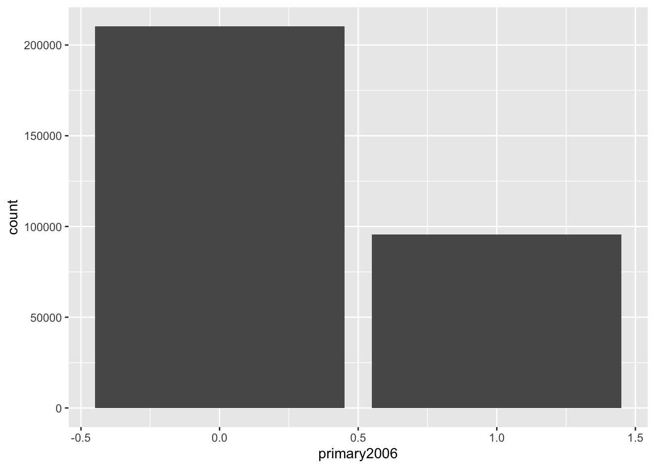
Notice that this gives these barplots in counts and automatically does that counting for us, but we might actually want to plot the proportions. To do this, we actually want to calculate the proportions using our tools above and then pass those geom_col (col for columns, I think??) which plots barplots when the heights of the bars are in the data itself:
social %>%
  group_by(primary2006) %>%
  summarize(prop = n() / nrow(social)) %>%
  ggplot(aes(x = primary2006, y = prop)) +
  geom_col()
## `summarise()` ungrouping output (override with `.groups` argument)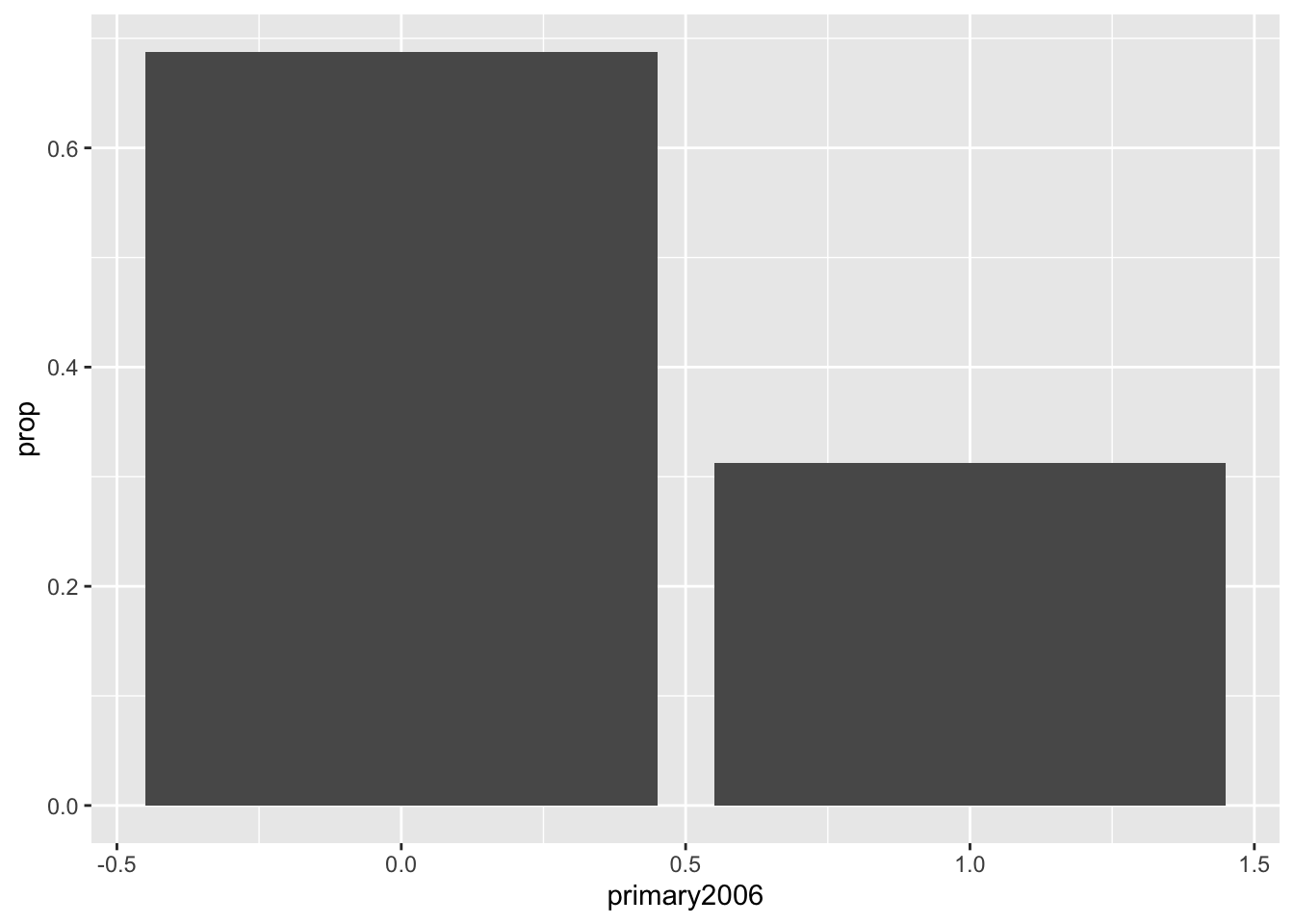
Now, notice that R seems to think the primary variable is a regular number and give us fractions on the x-axis. Now we can clean this up a bit by converting the variable of interest to a factor with informative labels and then adding our own axis labels:
social %>%
  mutate(
    p2006_fct = ifelse(primary2006 == 1, "Voted", "Abstained")
  ) %>%
  group_by(p2006_fct) %>%
  summarize(prop = n() / nrow(social)) %>%
  ggplot(aes(x = p2006_fct, y = prop)) +
  geom_col() +
  labs(x = "Voted in 2006 Primary", y = "Number of Respondents")
## `summarise()` ungrouping output (override with `.groups` argument)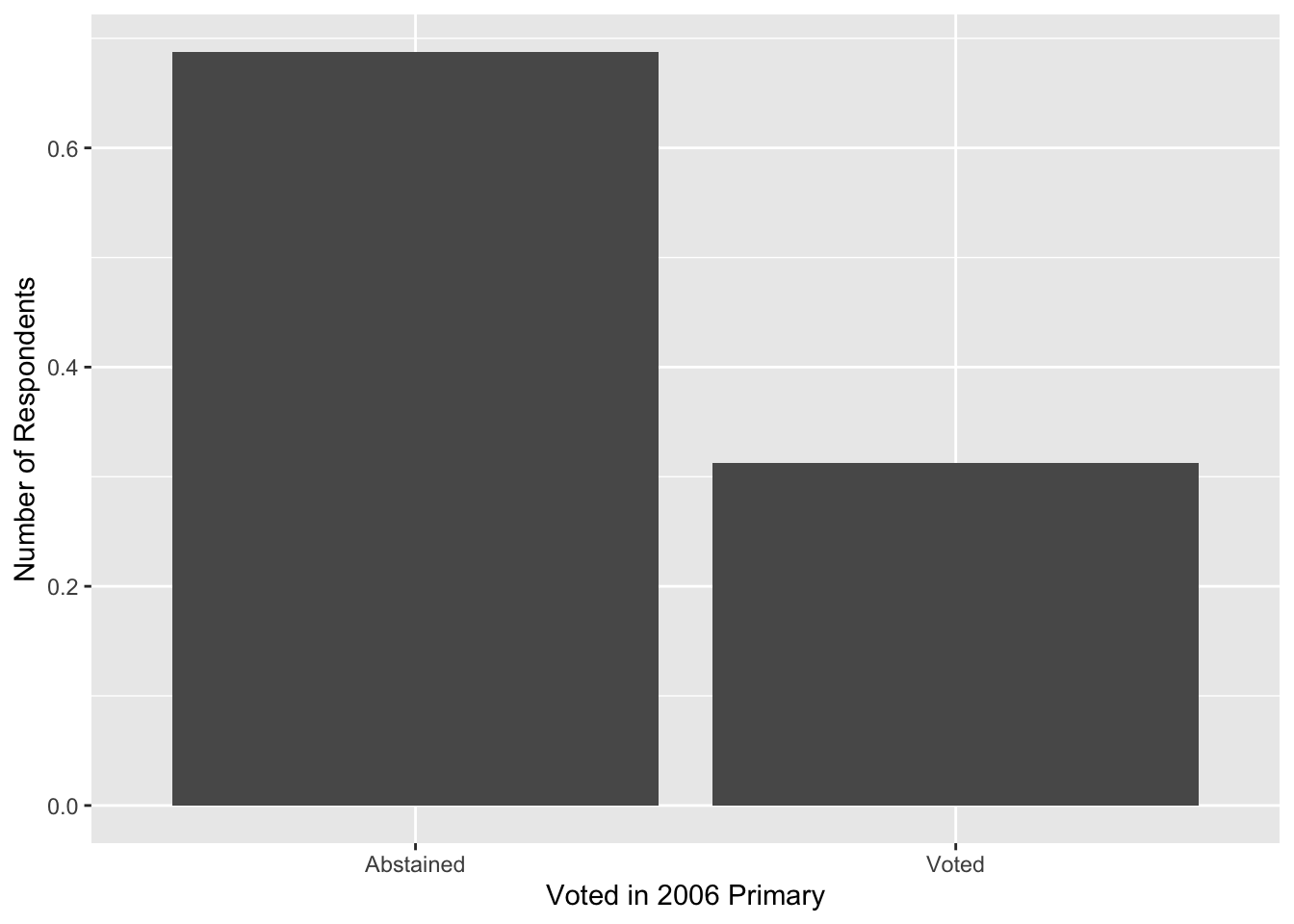
Histograms
We can make histograms with geom_histogram()
social$age <- 2006 - social$yearofbirth
ggplot(social, aes(x = age)) +
  geom_histogram()
## `stat_bin()` using `bins = 30`. Pick better value with `binwidth`.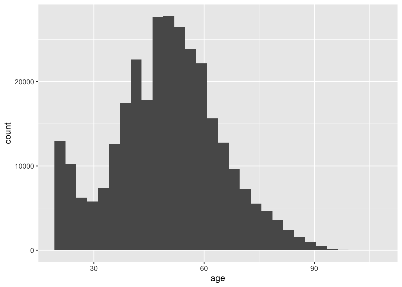
By default, geom_histogram() gives counts on the x-axis, but in QSS and in many applications it is easier to work with densities. This is because density histograms have a coherent interpretation in that the area of any particular bar in the histogram is the proportion of units in that bin of the variable. We can implement a density histogram using the following:
ggplot(social, aes(x = age)) +
  geom_histogram(aes(y = ..density..))
## `stat_bin()` using `bins = 30`. Pick better value with `binwidth`.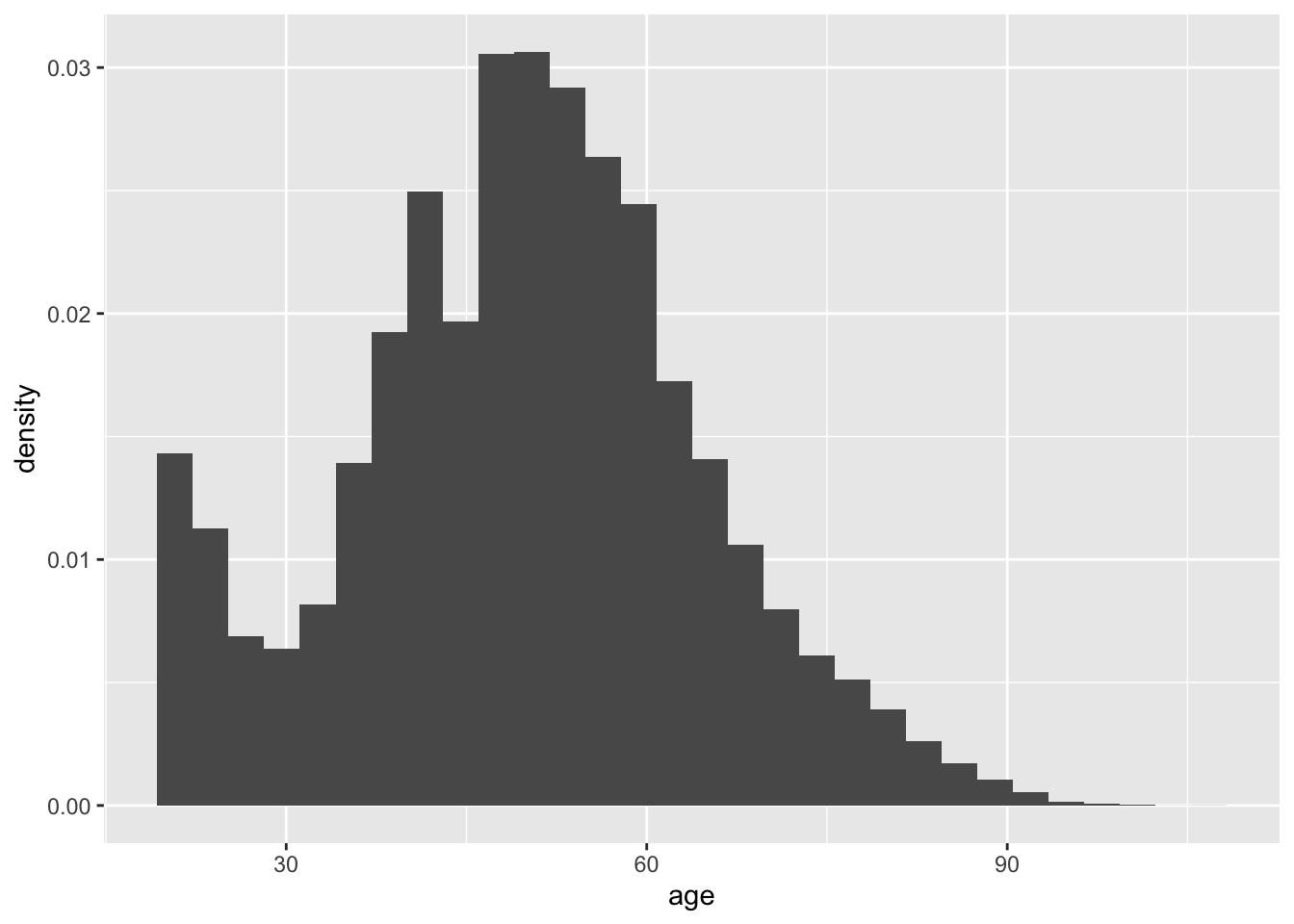
We can also make it fancy using various arguments. You may only want to use some of these.
ggplot(social, aes(x = age)) +
  geom_histogram(aes(y = ..density..), fill = "steelblue2", color = "white") +
  labs(x = "Age", y = "Density")
## `stat_bin()` using `bins = 30`. Pick better value with `binwidth`.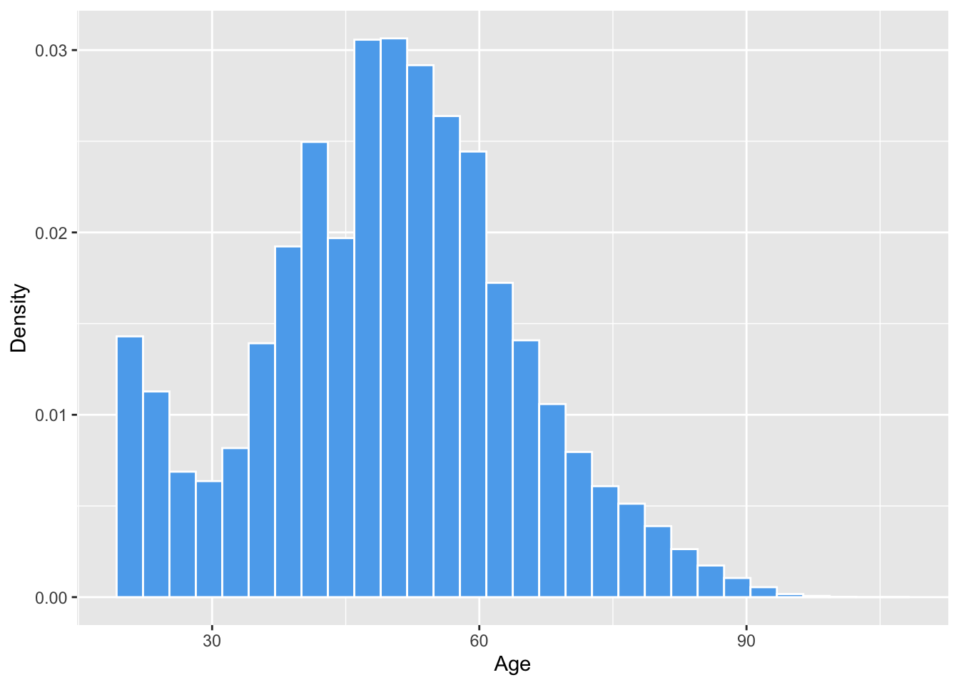
Boxplots
Here is the basic boxplot code with the defaults:
ggplot(social, aes(y = age)) +
  geom_boxplot()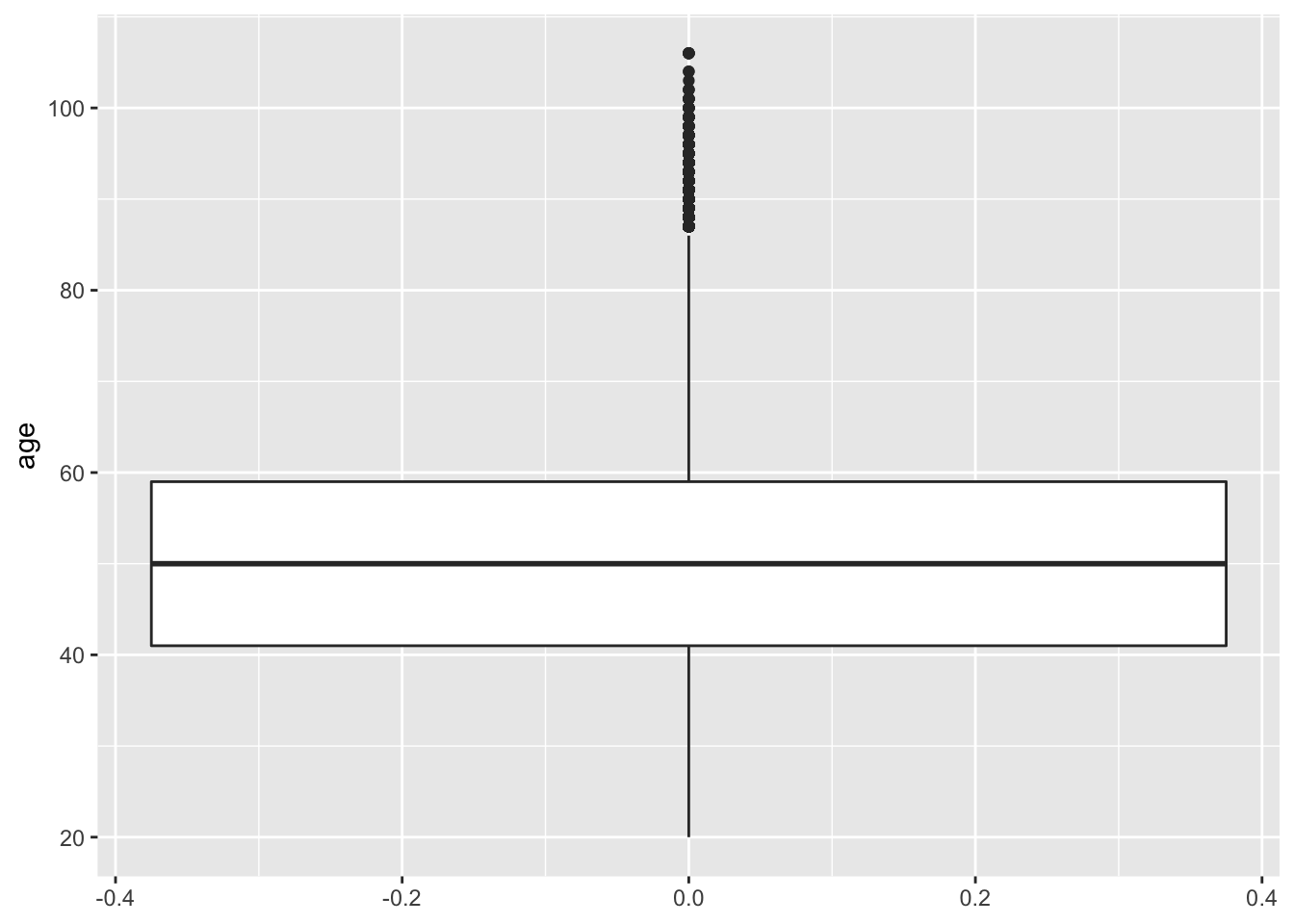
Wow, ugly! In order to get ggplot to ignore the x-axis and not plot random axis numbers, we can supply a dummy x variable which is just an empty string (""). Then, we can change the width to make it less fat and set the limits of the x-axis:
ggplot(social, aes(x = "", y = age)) +
  geom_boxplot(width = 0.2)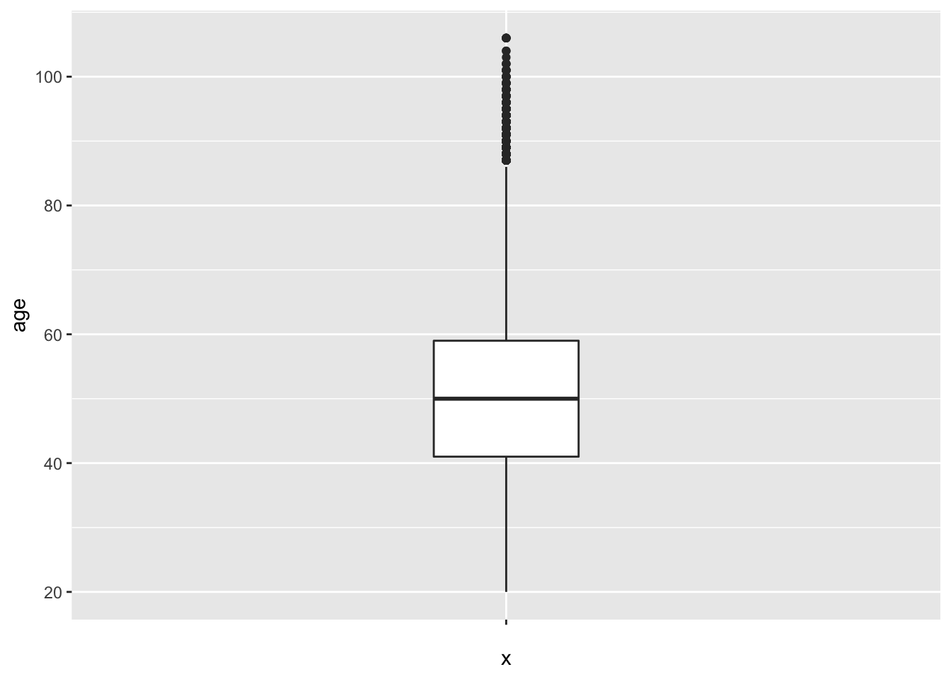
Missing data
Calculating means of vectors with missing values
To calculate the mean or sum of a vector with missing elements, using na.rm = TRUE as the final argument.
x <- c(1:5, NA)
x
## [1] 1 2 3 4 5 NAmean(x)## [1] NAmean(x, na.rm = TRUE)## [1] 3sum(x)## [1] NAsum(x, na.rm = TRUE)## [1] 15Testing if vector entries are missing or not
You can test if the entries of a vector are missing using the is.na() function:
x## [1] 1 2 3 4 5 NAis.na(x)## [1] FALSE FALSE FALSE FALSE FALSE TRUEYou can use the NOT operator ! to give you a vector that is TRUE when the vector is not missing:
!is.na(x)## [1] TRUE TRUE TRUE TRUE TRUE FALSERemoving NA values from a vector or data frame
There are a couple of ways to subset to a vector without the missing values.
x## [1] 1 2 3 4 5 NAna.omit(x)## [1] 1 2 3 4 5
## attr(,"na.action")
## [1] 6
## attr(,"class")
## [1] "omit"x[!is.na(x)]## [1] 1 2 3 4 5When applied to a data frame na.omit() removes any rows of the data frame that contain any missing values.
Week 4
Summarizing bivariate relationships
For this week, we’ll load the STAR data from the QSS package:
data(STAR, package = "qss")Scatterplots
To create a basic scatterplot, simply provide the variables corresponding the x and y axes:
ggplot(STAR, aes(x = g4math, g4reading)) +
  geom_point()
## Warning: Removed 3981 rows containing missing values (geom_point).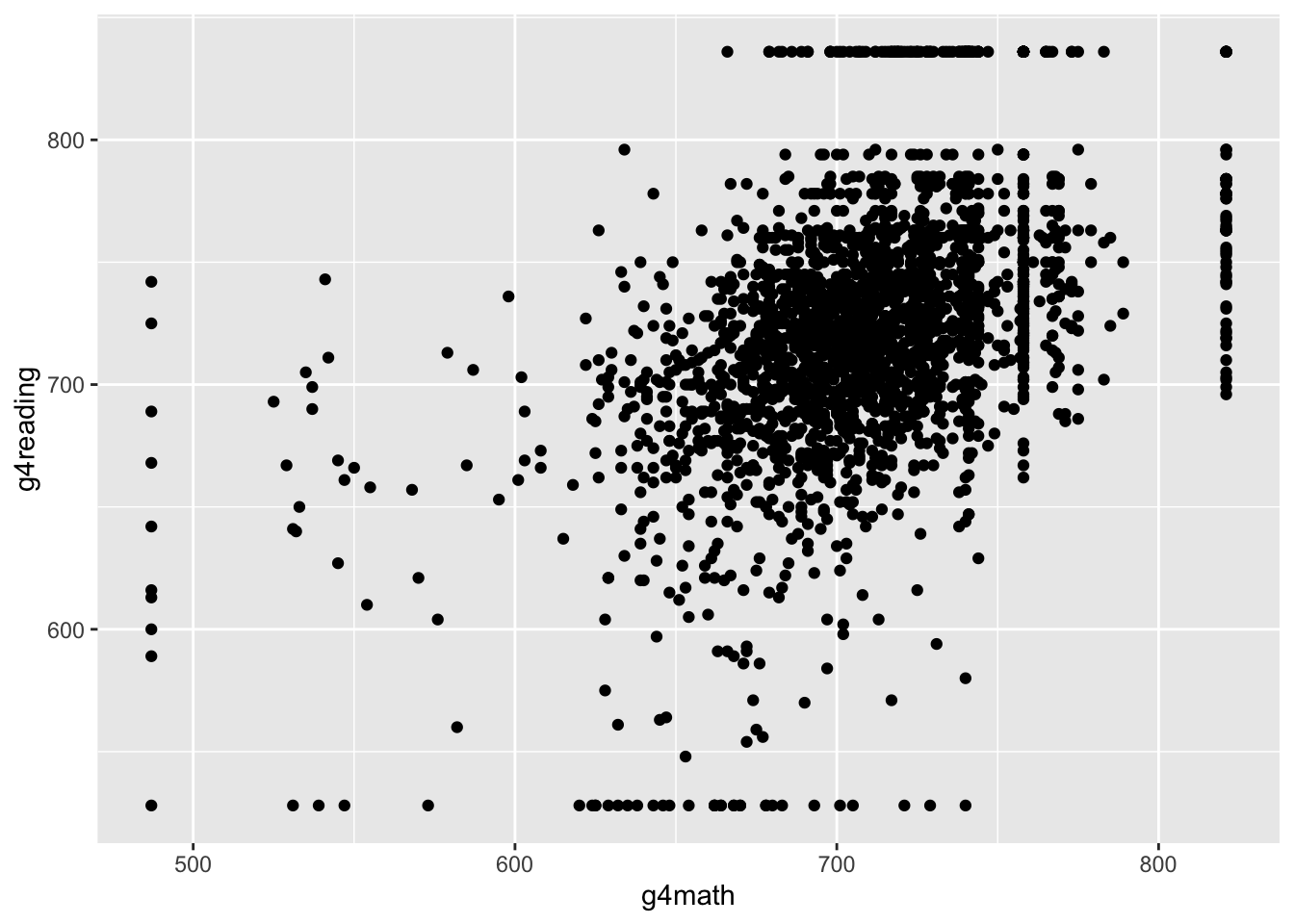
Of course, we can make these look quite a bit nicer:
ggplot(STAR, aes(x = g4math, g4reading)) +
  geom_point(color = "steelblue2") +
  labs(x = "Grade 4 Math Score", y = "Grade 4 Reading Score",
       title = "Reading and Math Score Relationship")
## Warning: Removed 3981 rows containing missing values (geom_point).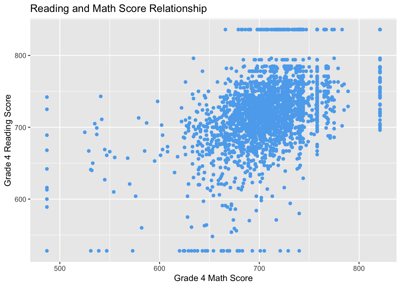
Making points more transparent in scatterplots
One thing to note is that when points are plotted over one another, solid points can look like a blob. In those cases, it might be reasonable to make the points more transparent. You can achieve this by using alpha argument in geom_point:
ggplot(STAR, aes(x = g4math, g4reading)) +
  geom_point(color = "steelblue2", alpha = 0.5) +
  labs(x = "Grade 4 Math Score", y = "Grade 4 Reading Score",
       title = "Reading and Math Score Relationship")
## Warning: Removed 3981 rows containing missing values (geom_point).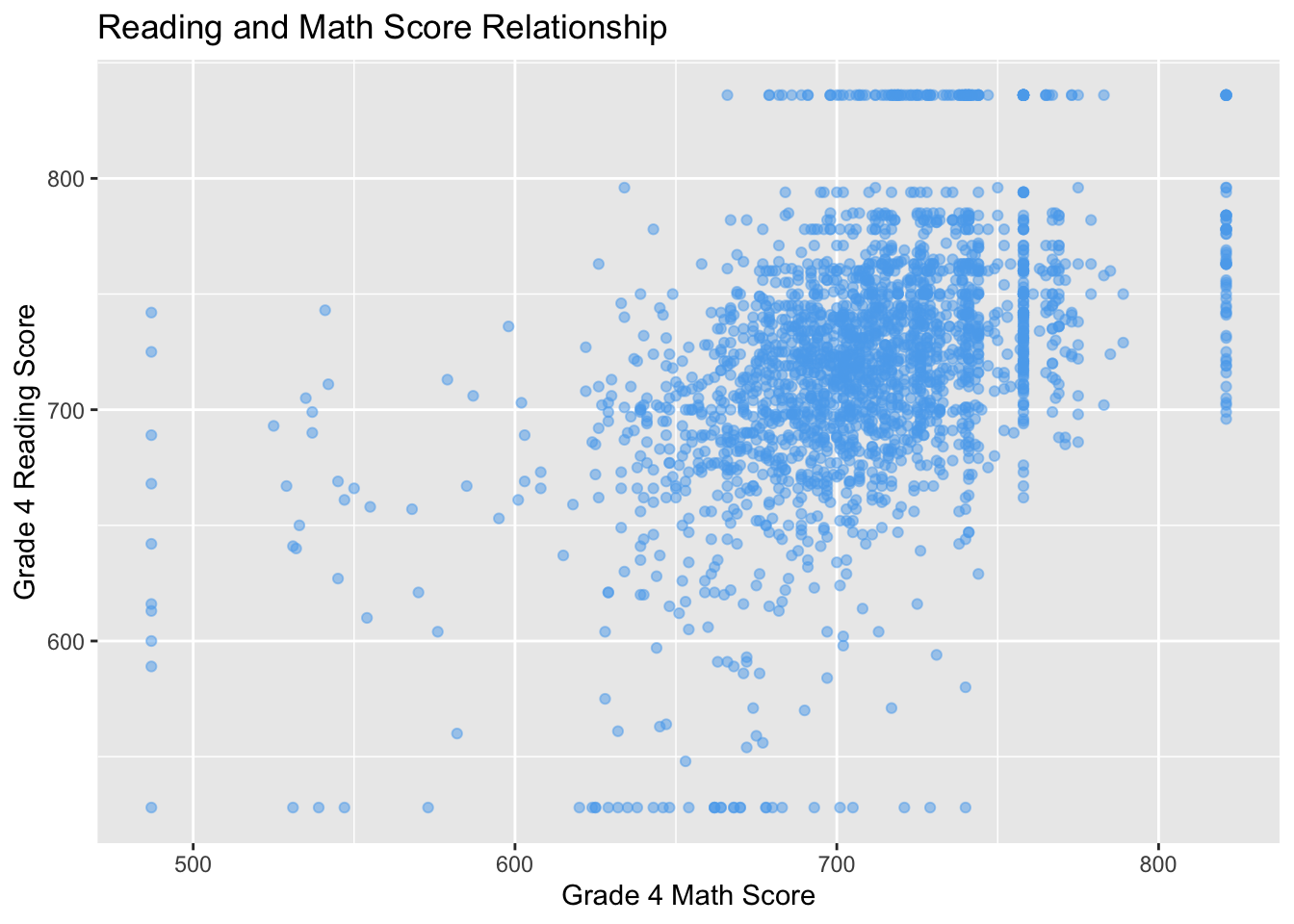
Here, setting the value of alpha in adjustcolor will change how transparent (0 being non-visible and 1 being full opaque). But now we can tell when points are plotted over one another more clearly.
Correlation
To take the correlation between two vectors of the same length, use the cor() function.
cor(STAR$g4math, STAR$g4reading)## [1] NAOops, there are missing values. Unlike other functions, you can’t use na.rm = TRUE here and instead you want to use use="pairwise":
cor(STAR$g4math, STAR$g4reading, use = "pairwise")## [1] 0.4694937Testing if entries of a vectors are equal to one of several values
In the STAR data, there is a variable yearssmall that describes how many years a student was in a small class type. This can take on 5 different values:
head(STAR$yearssmall)## [1] 0 0 0 4 0 0STAR %>% count(yearssmall)## yearssmall n
## 1 0 3957
## 2 1 768
## 3 2 390
## 4 3 353
## 5 4 857Maybe we want to compare units who are only have 0 or 1 year of small classes. We could do this with an OR statement:
STAR <- STAR %>%
  mutate(
    zero_or_one = ifelse(yearssmall == 0 | yearssmall == 1, 1, 0)
  )
head(STAR$zero_or_one)
## [1] 1 1 1 0 1 1This is a bit clunky, especially if we want to test for multiple categories. It is slightly easier to use the a %in% b syntax, which will check every entry of a to see if it is in b and give TRUE, otherwise it will give FALSE:
STAR <- STAR %>%
  mutate(
    zero_or_one = ifelse(yearssmall %in% c(0, 1), 1, 0)
  )
head(STAR$zero_or_one)
## [1] 1 1 1 0 1 1Boxplots by group
You might thin create boxplots by group in ggplot easiest by passing it as the group aesthetic:
ggplot(STAR, aes(group = classtype, y = g4math)) +
  geom_boxplot()
## Warning: Removed 3930 rows containing non-finite values (stat_boxplot).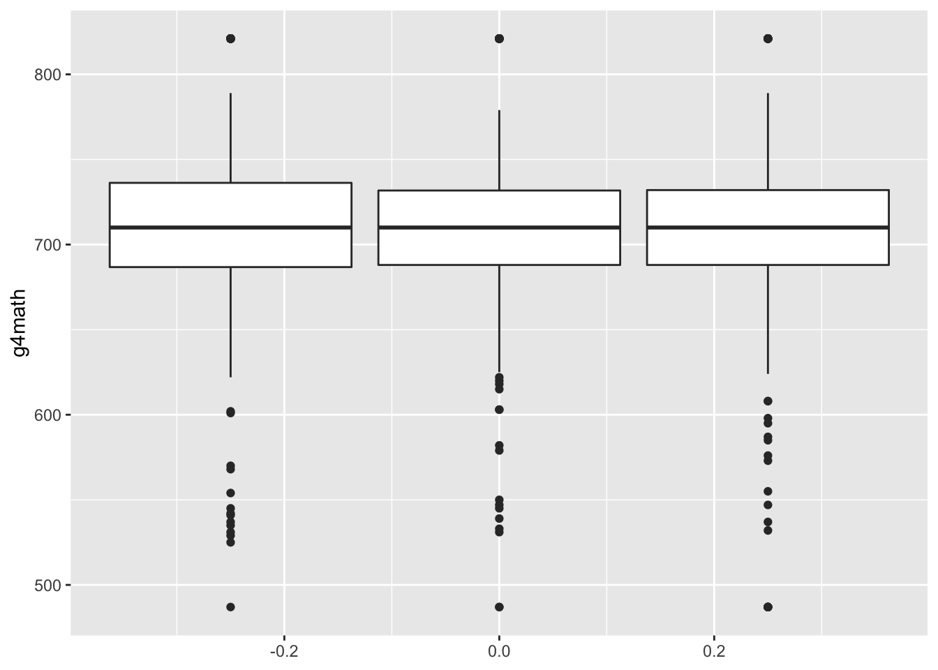
Of course, we can make this much nicer in appearance using the usual tricks. Note that the class size variable measures type of kindergarten class and takes on these values: small = 1, regular = 2, regular with aid = 3. One way to make this nicer is to first create a factor/character variable that has these labels and then pass this variable to the x aesthetic instead of groups:
STAR %>%
  mutate(
    class_fact = case_when(
      classtype == 1 ~ "Small",
      classtype == 2 ~ "Regular",
      classtype == 3 ~ "Regular w/ Aid"
    )
  ) %>%
ggplot(aes(x = class_fact, y = g4math)) +
  geom_boxplot() +
  labs(x = "Class type", y = "Grade 4 Math Scores")
## Warning: Removed 3930 rows containing non-finite values (stat_boxplot).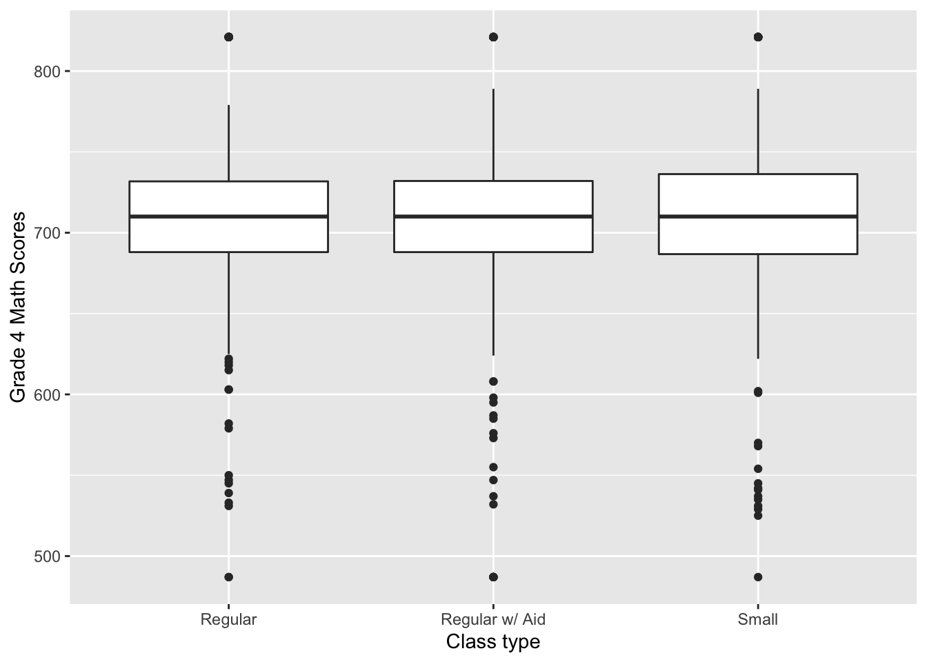
Q-Q plots
We can use the output from the qqplot() function to produce Q-Q plots. Note that we have to convert it to a data frame when passing to ggplot. You can also just plot with the qqplot() function
star_qq <- qqplot(x = STAR$g4math, y = STAR$g4reading, plot.it = FALSE)
ggplot(as.data.frame(star_qq), aes(x = x, y = y)) +
  geom_point()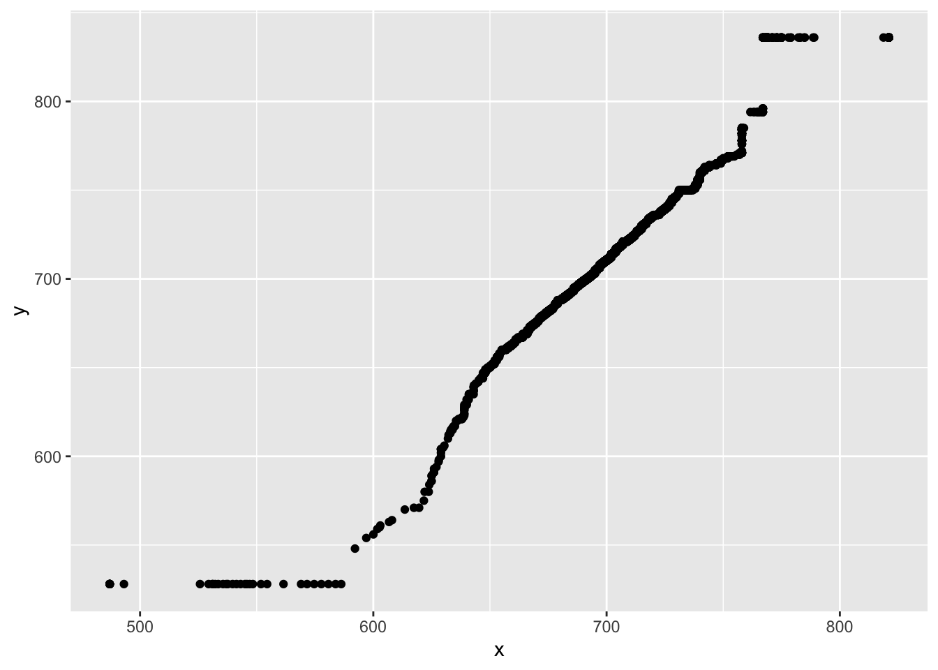
Producing lines on plots
You can produce straight lines on plots using the abline() command. There are three different ways to use it:
geom_vline(xintercept = 0): this will draw a vertical line at x = 0.geom_hline(yintercept = 0): this will draw a horizontal line at y = 0.geom_abline(intercept = 0, slope = 1): this will draw a straight line with y-intercept 0 and slope 1 (y = x).
We can use this in the Q-Q plot to draw a reference line:
star_qq <- qqplot(x = STAR$g4math, y = STAR$g4reading, plot.it = FALSE)
ggplot(as.data.frame(star_qq), aes(x = x, y = y)) +
  geom_point() +
  geom_abline(intercept = 0, slope = 1)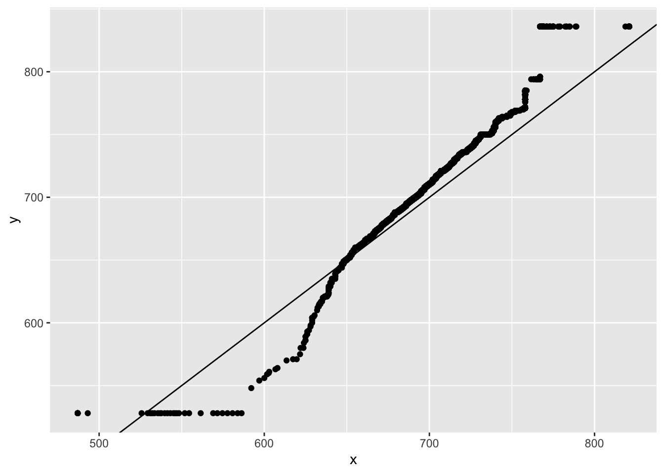
Week 5
Loops and conditionals
For loops
When coding for data analysis, we often have to perform repetitive tasks that change only in small ways. You could simply copy and paste the code for one of these task and manually change the code as needed, but this will get tedious very quickly. It will also make the code easier to read.
For example, suppose we wanted to calculate the mean of each column of the STAR data. We could achieve this by simply creating the vector by hand:
star_means <- c(mean(STAR$race, na.rm = TRUE),
                mean(STAR$classtype, na.rm = TRUE),
                mean(STAR$yearssmall, na.rm = TRUE),
                mean(STAR$hsgrad, na.rm = TRUE),
                mean(STAR$g4math, na.rm = TRUE),
                mean(STAR$g4reading, na.rm = TRUE))
star_means
## [1] 1.3407150 2.0523320 0.9541502 0.8332786 708.7766180 721.2477688This is a lot of code that does the same thing over and over again. Instead, we can use a loop to perform the same calculate applied to each column. To do this, we first need to create the placeholder vector where we will put all of the means, for which we use the rep function that creates a vector of a certain (or values) repeated some number of times. Then we start the loop using the for (i in X) construction. The X is a vector of values to iterate over and the i is the name of the iterator, a local variable in the loop that will give back current value of X in this iteration of the loop. Usually, X is of the form 1:n.
star_means <- rep(NA, times = ncol(STAR))
for (i in 1:ncol(STAR)) {
  star_means[i] <-  mean(STAR %>% pull(i), na.rm = TRUE)
}

star_means
## [1] 1.3407150 2.0523320 0.9541502 0.8332786 708.7766180 721.2477688 0.7470356We iterate over the columns of STAR so we use 1:ncol(STAR) in the setup of the loop and iterate through the column numbers/positions. We then subset the STAR data to that column and take its mean, assigning it to the ith position in the holder.
Printing output to the R console
You can print something to the R console using the cat() command. Note that you need to add at least one \n at the end of the string so that the next thing to print will be on the next line.
cat("hello world!\n")## hello world!if statements
If statements are a powerful computing tool that allow us to execute code only if some conditions hold. We might implement it like this:
if (condition) {
  [code to evaluate]
}
For instance, let’s have R tell us if we have a negative number:
if (x < 0) {
  cat("Hey! That's a negative!\n")
}
## Hey! That's a negative!cat("Wow, we've reached the end!\n")## Wow, we've reached the end!Compare this to the same code, but given a positive number:
x <- 4
if (x < 0) {
  cat("Hey! That's a negative!\n")
}
cat("Wow, we've reached the end!\n")
## Wow, we've reached the end!if/else statements
You can use the if {} else {} construct to have a set of fallback code that executes if the condition is not met. Continuing our theme:
x <- -4
if (x < 0) {
  cat("Hey! That's a negative!\n")
} else {
  cat("Whoa! It's positive!\n")
}
## Hey! That's a negative!x <- 4
if (x < 0) {
cat("Hey! That's a negative!\n")
} else {
cat("Whoa! It's positive!\n")
}## Whoa! It's positive!Linear regression
We’ll use the leader assassinations data from the QSS book and the lectures.
data(leaders, package = "qss")Fitting a linear regression model
First, we’ll regress the polity (aka democracy) score after the assassination attempt on the same score before:
fit <- lm(polityafter ~ politybefore, data = leaders)
fit
##
## Call:
## lm(formula = polityafter ~ politybefore, data = leaders)
##
## Coefficients:
## (Intercept) politybefore
## -0.3764 0.8386Obtaining the vector of estimated regression coefficients
coef(fit)## (Intercept) politybefore
## -0.3764159 0.8386199Obtaining a vector of fitted/predicted values from the regression
head(fitted(fit))## 1 2 3 4 5 6
## -5.4081352 -5.4081352 -5.4081352 -0.3764159 -7.9239949 -7.9239949Adding a regression line to a plot
You can use the abline() function with the lm() output to add a regression line to a plot:
ggplot(leaders, aes(x = politybefore, y = polityafter)) +
  geom_point(color = "steelblue2", alpha = 0.5) +
  labs(x = "Polity Before", y = "Polity After") +
  geom_smooth(method = "lm", color = "indianred")
## `geom_smooth()` using formula 'y ~ x'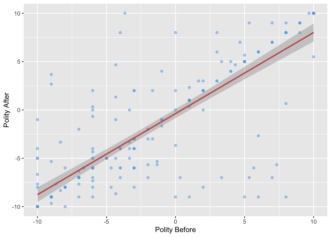
Obtaining the vector of residuals
head(residuals(fit))## 1 2 3 4 5 6
## -0.5918648 -1.9251981 -2.5918648 -8.6235841 -1.0760051 -1.0760051Week 6
Multiple regression
Fitting a linear model with multiple predictors
We can have multiple predictors in our regression by separating them on the right-hand side by the + symbol:
mult_fit <- lm(polityafter ~ politybefore + interwarbefore + civilwarbefore,
               data = leaders)
mult_fit
##
## Call:
## lm(formula = polityafter ~ politybefore + interwarbefore + civilwarbefore,
## data = leaders)
##
## Coefficients:
## (Intercept) politybefore interwarbefore civilwarbefore
## -0.7110 0.8342 1.5337 0.1830Model fit
Accessing the R squared
You can access the \(R^2\) of the regression using the summary() function:
summary(mult_fit)$r.squared## [1] 0.69464Accessing the adjusted R squared
summary(mult_fit)$adj.r.squared## [1] 0.6909161Week 7
Interactions
We can see if the relationship between polityafter and politybefore is different when there is a civil war before or not with an interaction. Interactions between two independent variable can be specified by putting a * between them:
int_fit <- lm(polityafter ~ politybefore * civilwarbefore, data = leaders)
int_fit
##
## Call:
## lm(formula = polityafter ~ politybefore * civilwarbefore, data = leaders)
##
## Coefficients:
## (Intercept) politybefore civilwarbefore
## -0.4302 0.8233 0.2823
## politybefore:civilwarbefore
## 0.0922Nonlinear relationships
To demonstrate the nonlinear relationships, let’s look at the relationship between democracy scores after the assassination attempt and the age of the leader. We’ll fit a parabola using I() to wrap the squared term, indicating to R to interpret the math expression literally.
nonlin_fit <- lm(polityafter ~ age + I(age ^ 2), data = leaders)
nonlin_fit
##
## Call:
## lm(formula = polityafter ~ age + I(age^2), data = leaders)
##
## Coefficients:
## (Intercept) age I(age^2)
## -7.9796587 0.0978674 0.0003627Predicted values from a regression
We can get predicted values from a regression output by passing a new data frame with the values of the independent variables we want a predictor for. For example, suppose we wanted to get the predicted values of the polity score after for each leader age between 18 and 81. We could do the following:
age_vals <- 18:81
age_preds <- predict(nonlin_fit, newdata = data.frame(age = age_vals))
We can plot predicted values a bit easier using ggplot and geom_smooth where now we give a formula that indicates that we want the squared term along with the linear term.
ggplot(leaders, aes(x = age, y = polityafter)) +
  geom_smooth(method = "lm", formula = y ~ x + I(x ^ 2))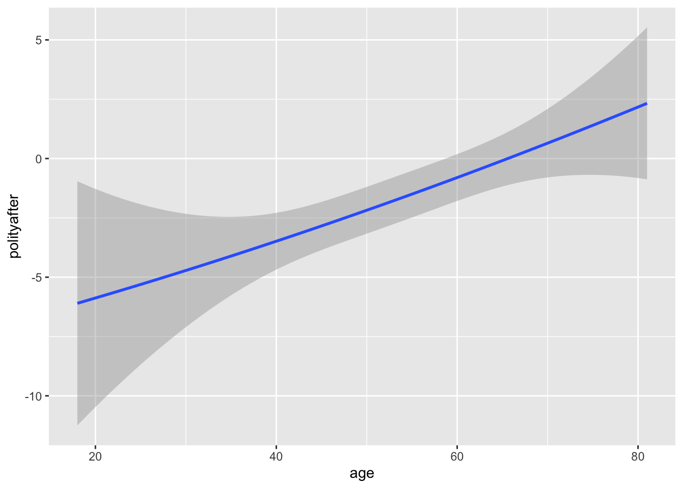
Week 8
Sampling from a vector without replacement
You can randomly draw from a vector of objects using the sample() function. For example, to randomly select four from the years 2000 to 2020, we can do the following:
sample(x = 2000:2020, size = 4, replace = FALSE)## [1] 2018 2008 2013 2011By default, sample will sample each item with equal probability.
Sampling from a vector with replacement
Suppose we wanted to use R to randomly generate a 10-letter word. There is a built-in vector in R called letters that is just a vector of the alphabet. Here we want to be able to reuse letters so we set replace = TRUE:
letters## [1] "a" "b" "c" "d" "e" "f" "g" "h" "i" "j" "k" "l" "m" "n" "o" "p" "q" "r" "s" "t" "u"
## [22] "v" "w" "x" "y" "z"sample(letters, size = 10, replace = TRUE)## [1] "n" "i" "m" "z" "s" "k" "s" "b" "v" "k"Here you can see that both k and s are repeated, though this word doesn’t make any sense!
Week 9
Probability Distributions
Drawing binomial random variables
You can sample from the binomial distribution with a specific set of parameters using the rbinom() function. Suppose we wanted to sample the number of heads in 15 draws of an unfair coin with probability 0.25 of landing heads.
rbinom(n = 5, size = 15, prob = 0.25)## [1] 5 2 4 3 5If we call the same function again, we will get a different set of random draws:
rbinom(n = 5, size = 15, prob = 0.25)## [1] 2 4 5 6 6Drawing a Bernoulli random variable
To draw a Bernoulli random, simply use rbinom() with size = 1.
Calculating the probability mass function of a binomial
You can calculate the probability of any possible value of a binomial random variable using the dbinom() function:
dbinom(x = 8, size = 15, prob = 0.25)## [1] 0.01310682Drawing a normal random variable
You can use the rnorm() function to draw from a normal random variable. Note that you pass it the standard deviation, not the variance of the distribution you want.
rnorm(n = 5, mean = 4, sd = 3)## [1] 5.323501 3.431394 1.923554 5.991246 5.870274Week 11
Hypothesis tests
Proportion test
Suppose we had a sample where 440 out of 1000 said they would support Trump and we wanted to see if that sample proportion of 0.44 was significantly different than the true support among voters (0.475). We can do this by hand as or with the prop.test() function:
prop.test(440, n = 1000, p = 0.475)##
## 1-sample proportions test with continuity correction
##
## data: 440 out of 1000, null probability 0.475
## X-squared = 4.7729, df = 1, p-value = 0.02891
## alternative hypothesis: true p is not equal to 0.475
## 95 percent confidence interval:
## 0.4090275 0.4714392
## sample estimates:
## p
## 0.44This also gives a confidence interval as well:
prop.test(440, n = 1000, p = 0.475)$conf.int## [1] 0.4090275 0.4714392
## attr(,"conf.level")
## [1] 0.95Both of these use the normal approximation, but you can also do a test leveraging the exact binomial distribution:
binom.test(440, n = 1000, p = 0.475)##
## Exact binomial test
##
## data: 440 and 1000
## number of successes = 440, number of trials = 1000, p-value = 0.02669
## alternative hypothesis: true probability of success is not equal to 0.475
## 95 percent confidence interval:
## 0.4089497 0.4714046
## sample estimates:
## probability of success
## 0.44Tests of a single mean
Any time we want to test a sample mean, the standard practice is to conduct a t-test, even though a z-test might be justified by the central limit theorem. Thus, the common way to do a one-sample test is with t.test. For example, in the STAR data on small class sizes, we might want to test if the reading scores in our data have the same mean as the national average of 710. We can do that with the following:
t.test(STAR$g4reading, mu = 710)##
## One Sample t-test
##
## data: STAR$g4reading
## t = 10.407, df = 2352, p-value < 2.2e-16
## alternative hypothesis: true mean is not equal to 710
## 95 percent confidence interval:
## 719.1284 723.3671
## sample estimates:
## mean of x
## 721.2478And we can also get confidence intervals from this procedure as well:
t.test(STAR$g4reading, mu = 710)$conf.int## [1] 719.1284 723.3671
## attr(,"conf.level")
## [1] 0.95Tests comparing two sample means
If we want to compare the means of a continuous variable as a function of some binary variable, we can use a formula in the t.test function. In particular, we can compare the STAR reading scores by class type (subsetting to the small 1 and regular 2 class types). The formula should be y ~ x where y the variable whose mean we want and x is a variable that defines the groups.
t.test(g4reading ~ classtype, data = STAR,
       subset = classtype %in% c(1,2))
##
## Welch Two Sample t-test
##
## data: g4reading by classtype
## t = 1.3195, df = 1541.2, p-value = 0.1872
## alternative hypothesis: true difference in means is not equal to 0
## 95 percent confidence interval:
## -1.703591 8.706055
## sample estimates:
## mean in group 1 mean in group 2
## 723.3912 719.8900We can perform the same test using a different set of arguments:
t.test(STAR$g4reading[STAR$classtype == 1],
       STAR$g4reading[STAR$classtype == 2])
##
## Welch Two Sample t-test
##
## data: STAR$g4reading[STAR$classtype == 1] and STAR$g4reading[STAR$classtype == 2]
## t = 1.3195, df = 1541.2, p-value = 0.1872
## alternative hypothesis: true difference in means is not equal to 0
## 95 percent confidence interval:
## -1.703591 8.706055
## sample estimates:
## mean of x mean of y
## 723.3912 719.8900Tests comparing two sample proportions
You can also use the prop.test function to test differences in proportions. In the social pressure mailer example, we can subset to just the Neighbors arm and then create a cross-tab with the treatment on the rows and the outcome of interest in the columns. When we pass this to the prop.test function, it will perform the test of the differences in proportions.
test_tab <- social %>%
  filter(messages %in% c("Neighbors", "Control")) %>%
  group_by(messages, primary2006) %>%
  summarize(count = n()) %>%
  pivot_wider(names_from = primary2006, values_from = count) %>%
  ungroup() %>%
  select(`1`, `0`)
## `summarise()` regrouping output by 'messages' (override with `.groups` argument)test_tab## # A tibble: 2 x 2
## `1` `0`
## <int> <int>
## 1 56730 134513
## 2 14438 23763prop.test(as.matrix(test_tab))##
## 2-sample test for equality of proportions with continuity correction
##
## data: as.matrix(test_tab)
## X-squared = 983.46, df = 1, p-value < 2.2e-16
## alternative hypothesis: two.sided
## 95 percent confidence interval:
## -0.08660129 -0.07601853
## sample estimates:
## prop 1 prop 2
## 0.2966383 0.3779482